The Johnson-Lindenstrauss lemma for the brave

If you are interested in dimensionality reduction, chances are that you have come across the Johnson-Lindenstrauss lemma. I learned about it while studying the Linformer paper, which contains a result on dimensionality reduction for the Transformer. Essentially, they prove that self-attention is low-rank, by appealing to the Johnson-Lindenstrauss lemma.

Online, you can find many elementary proofs of this lemma. Unfortunately, most of them have sacrificed some intuition and generality in order to simplify the proofs, for instance by using Gaussian distributions. I was left a bit unsatisfied by this, so I started to study the proof in the original paper ¹. According to the eponymous authors, the lemma is "a simple consequence of the isoperimetric inequality for the \(n\)-sphere". But what does that mean? That is the content of this post.

Statement of the lemma

The Johnson-Lindenstrauss lemma says the following. Given an integer \(N\), there is a small dimension \(k\), such that for any dimension \(n\) and every every \(N\) points \({x_1, \dots, x_N} \in \mathbb{R}^n\), there exists a linear map \[ L : \mathbb{R}^n \to \mathbb{R}^k \] which is very close to preserving all distances between each pair of the \(N\) points. The lemma specifies how small \(k\) can be, namely \(O(K(\tau)\log N)\). Here \(\tau\) makes precise what it means to be close to distance-preserving. We will actually see that \(K(\tau)\) can be taken to be \(1/\tau^2\).

The formal statement of the lemma goes like this.

Lemma. Let \(0 < \tau < 1\). Then there is a constant \(K > 0\) so that if \({x_1, \dots, x_N} \in \mathbb{R}^n\) for \(N \geq 2\) and \(k \geq \lceil K \log N / \tau^2 \rceil\), there is a linear map \(L : \mathbb{R}^n \to \mathbb{R}^k\) such that \[ (1-\tau) \lVert x_i - x_j \rVert \leq \lVert L(x_i) - L(x_j) \rVert \leq (1+\tau) \lVert x_i - x_j\rVert\] for all \(1 \leq i , j \leq N\).

Before I start with the proof, observe that is enough to find \(L\) which satisfies for all \(i, j\): \[ (1-\tau) M \lVert x_i - x_j \rVert \leq \lVert L(x_i) - L(x_j) \rVert \leq (1+\tau) M\lVert x_i - x_j\rVert. \] For some constant \(M\). Because then \(L\) can just be rescaled to satisfy the condition of the lemma. So it is enough to focus on this slightly more relaxed statement.

Like its many adaptations, the original proof is probabilistic. That means that the strategy is to show that a random \(L\) (sampled from a suitable space) satisfies the (relaxed) statement with nonzero probability. Therefore, there must exist one. A tighter estimate for the probability is nice to have, because this will give an estimate of how quickly you can find a suitable witness. It turns out that you can actually find one in randomized polynomial time, which is reassuring for applications in computer science.

Contribution

Besides presenting the original proof, I will derive an explicit witness \(K\). Such a witness is not given in the original papers (at least not one that works for small \(N\) also). To obtain a reasonably low value for \(K\), I did some of the estimates differently. This value is nice to have because there are different ones around in literature, and not all of them apply to the lemma in the form stated here (see also the remark at the end). I do think there is room for improvement in the value I'm getting currently!

Summary of the proof

Before we dive in, we can summarise the structure of the proof in the following steps:

1. Restate the goal to a probability that a certain seminorm on \(\mathbb{R}^n\) is almost constant on a finite set of points on the \((n-1)\)-sphere.
2. Estimate this probability from below using the isoperimetric inequality, which is the fact that a 'cap' on the \((n-1)\)-sphere has the lowest perimeter-to-area ratio of all subsurfaces of the \((n-1)\)-sphere.
3. Find a lower bound for the constant in (1.) and use it to show that the probability is nonzero.
4. Conclude.

To make the proof more accessible, I have replaced all measure-theoretic notation by the more intuitive probabilities or (normalized) surface area. For measurable subsets \(A \subset S^{n-1}\) of the \((n-1)\)-sphere I denote their normalized 'surface area' by \(\text{vol}_{n-1}(A)\), referring to the unique rotation invariant normalized (or probability) Borel measure on \(S^{n-1}\). But you can think of it as surface area on a sphere.

The proof

As a preliminary, we need a definition of random linear map \(L : \mathbb{R}^n \to \mathbb{R}^k\), which we will just interpret as a rank \(k\) matrix \(L : \mathbb{R}^n \to \mathbb{R}^n\). Many elementary proofs use a Gaussian distribution on the components of the matrix. But the original paper does something a bit more elegant.

Namely, although there is no standard notion of random matrix, there is a canonical choice of random orthogonal matrix. Recall that a matrix \(U\) is orthogonal if \(U^TU = UU^T = 1\). These are the linear operations on \(\mathbb{R}^n\) that preserve inner products. They can be thought of as compositions of rotations around an axis and reflections along an axis. And it turns out that there is a well-defined and unique notion of random variable with values in \(O(n)\), satisfying some nice conditions. For instance, this notion of randomness is invariant along postcomposition with a fixed orthogonal transformation. The mathematical reason behind this is that \(O(n)\) forms a compact Lie group on which there is a unique normalized Haar measure. But for the rest of this post, we will only need the fact that orthogonal matrices can be sampled and that they enjoy rotation invariance.

We can use this to obtain a notion of 'random rank \(k\) projection' matrix \(L\) as follows. Suppose \(U \in O(n)\) is a random orthogonal matrix. Then define \[ L := U^TQU \] where \(Q\) is the projection on the first \(k\) coordinates. That's it! Note that not all matrices have this shape. But to find a matrix, we will see that it is enough to sample \(L\) in this way. We can now take our problem to the unit sphere.

1. Reformulation to a problem on the \((n-1)\)-sphere

We use the following notation for taking the (scaled) norm of the first \(k\) components of an \(n\)-vector: \[ r(y) = b \lVert Qy\rVert = b\sqrt{\sum_{i=1}^k y_i^2} \] where \(b > 0\) could be anything for now. Observe that \(r(y) \leq b \lVert y\rVert\).

The difference vectors \(x_i - x_j\) of the \(n\) points can be projected down to the surface of the unit ball, the sphere \(S^{n-1}\): \[ B = \left\{\frac{x_i - x_j}{\lVert x_i - x_j\rVert} : 1 \leq i < j \leq n\right\} \subset S^{n-1} \] Then, our goal can be formulated as follows. We want to find \(U \in O(n)\), such that for every \(y \in B\), we have: \[ (1-\tau)M \leq r(Uy) \leq (1+\tau)M \] for some constant \(M\). This can be interpreted as: given a set of points on the \((n-1)\)-sphere, find an orthogonal transformation so that the norms of the first \(k\) coordinates of all transformed points are close to the same constant. In the following, we will show that a random \(U \in O(n)\) satisfies the condition with positive probability.

2. Using isoperimetric inequality to estimate probability

To make things easier, we will first study \(r(y)\) for \(y\) randomly sampled from \(S^{n-1}\). This is the same thing as studying \(r(Uy_0)\) for fixed \(y_0 \in S^{n-1}\) and \(U \in O(n)\) random, thanks to rotation invariance.

Seminorms concentrated near their median

The function \(r\) defined above defines a seminorm on \(\mathbb{R}^{n}\). The precursor paper ² proves an interesting property about (semi)norms that satisfy \(r(y) \leq b \lVert y\rVert\) for some bound \(b\), like our \(r\). Namely, their value for random vectors on the unit sphere is increasingly concentrated around their median as \(n\) increases.

With the median \(M_r\) of \(r\), we mean any value (there exists one) \(M_r\) such that \[ \mathbb{P}(r(y) \geq M_r) \geq \frac{1}{2} \text{ and }\mathbb{P}(r(y) \leq M_r) \geq \frac{1}{2} \] (This is the slightly awkward mathematical definition of median).

For a subset \(A \subset S^{n-1}\), denote by \(A_\epsilon\) the set of points in \(S^{n-1}\) that have (geodesic) distance \(<\epsilon\) to some point in \(A\). In the next section, we will estimate the probability \[ \mathbb{P}(y \in A_\epsilon) \] for a suitable set \(A\) from below, using a geometric fact about spheres.

Isoperimetric inequality for spheres

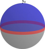
Specifically, the authors make use of the isoperimetric inequality. This is the intuitively (at least for \(n = 3\)) obvious fact that a 'cap' on the \((n-1)\)-sphere has the smallest perimeter-to-area ratio of all possible measurable subsurfaces of the \((n-1)\)-sphere. Denote by \(B(r,x_0)\) the 'cap' centred at a point \(x_0\) of radius \(r\) (measured in radians, so \(0 < r < \pi\)). For \(n = 3\) and \(r=\pi/2\), this is the cap which covers half the sphere, drawn as the blue area on the surface of the sphere below. The red band indicates all points in the complement that are a geodesic distance \(<\epsilon\) from \(B(r,x_0)\). Both areas combined form the set \(B(r,x_0)_\epsilon\).

Then we use the isoperimetric inequality in the following form: when \(A\) is a subsurface with \[ \text{vol}_{n-1}(A) = \text{vol}_{n-1}(B(r,x_0)) \] then \[ \text{vol}_{n-1}(A_\epsilon) \geq \text{vol}_{n-1}(B(r,x_0)_\epsilon). \] For all \(\epsilon > 0\). This brings us to the median. Suppose \(A^+ = \{y \in S^{n-1} \mid r(y) \geq M_r\}\), and let \(B(\pi/2,x_0)\) be the 'half cap' as above. Then for all \(\epsilon\): \[ \text{vol}_{n-1}(A^+_\epsilon) \geq \text{vol}_{n-1}(B(\pi/2, x_0)_\epsilon) \] by the isoperimetric inequality. For \(A^- = \{y \in S^{n-1} \mid r(y) \leq M_r \}\), we have a similar estimate \[ \text{vol}_{n-1}(A^-_\epsilon) \geq \text{vol}_{n-1}(B(\pi/2, x_0)_\epsilon). \] So for the join of the complements of the two areas, we get: \[ \begin{aligned} \text{vol}_{n-1}(S^{n-1} \setminus A^-_\epsilon \cup S^{n-1} \setminus A^+_\epsilon) &\leq 2(\text{vol}_{n-1}(S^{n-1}) - \text{vol}_{n-1}(B(\pi/2, x_0)_\epsilon))\\ &= 2(1 - \text{vol}_{n-1}(B(\pi/2, s_0)_{\epsilon})) \end{aligned} \] But the left-hand side is precisely the area \(\text{vol}_{n-1}(S^{n-1} \setminus A_\epsilon)\), where \(A := \{y \in S^{n-1} \mid r(y) = M_r\}\). Hence we obtain our estimate as: \[ \text{vol}_{n-1}(A_\epsilon) \geq 2\cdot \text{vol}_{n-1}(B(\pi/2, x_0)_\epsilon) - 1 \] which in terms of probabilities of random points on the sphere becomes \[ \mathbb{P}(y \in A_\epsilon) \geq 2\cdot \mathbb{P}(y \in B(\pi/2,x_0)_\epsilon) - 1. \] This result is also known as Levy's lemma. Now since the geodesic distance to \(A\) is always bigger than the euclidean distance, this implies: \[ \mathbb{P}(M_r - b\epsilon \leq r(y) \leq M_r + b \epsilon) \geq 2\cdot \mathbb{P}(y \in B(\pi/2,x_0)_\epsilon) - 1 \] (you have to use the triangle inequality twice - here we need that \(r\) is a seminorm).

Now, one can evaluate the right-hand side using ordinary calculus. I will not go over the calculations, but the authors use it to rewrite the estimate as \[ \mathbb{P}(y \in A_\epsilon) \geq 2 \gamma_n\int_{0}^\epsilon \cos^{n-2}t dt \] and then estimate \[ 2\gamma_n\int_0^\epsilon \cos^{n-2}t dt \geq 1 - 4 e^{-n\epsilon^2/2}. \] The curious property this exhibits is that for higher dimensional spheres, most of their 'surface area' is centred around their 'perimeter'. That is, for high \(n\), the normalized area \[ \text{vol}_{n-1}(B(x_0, \pi/2)_\epsilon) \] gets close to \(1\), even for small \(\epsilon\), contrasting the intuition from the illustration above. For us, the estimate implies \[ \mathbb{P}(M_r - b\epsilon \leq r(y) \leq M_r + b \epsilon) \geq 1 - 4 e^{-n\epsilon^2/2}. \] Note this holds for all \(\epsilon\). Now say we can find a lower bound for \(M_r\), e.g. \(L \leq M_r\) for a constant \(L\). Then by letting \(\epsilon := \tau L/b\), we get: \[ \begin{aligned} &\mathbb{P}((1-\tau)M_r \leq r(Uy) \leq (1+\tau)M_r) \\ &\geq \mathbb{P}(M_r - \tau L \leq r(Uy) \leq M_r + \tau L) \\ &\geq \mathbb{P}(M_r - \epsilon b \leq r(Uy) \leq M_r + \epsilon b) \geq 1 - 4 e^{-n\epsilon^2/2} \\ &\geq 1 - 4 e^{-n\tau^2 L^2 / 2 b^2} \end{aligned} \] For a fixed \(y\) and \(U \in O(n)\) random. But recall we want this estimate to be greater than zero for all \(y \in B\), a set of \(N(N+1)/2\) points (all pairs). In the worst case, each \(y \in B\) has its own region of \(U\)'s where the above condition is violated. This gives a new estimate: \[ \begin{aligned} &\mathbb{P}((1-\tau)M_r \leq r(Uy) \leq (1+\tau)M_r \text{ for all } y \in B) \\ &\geq 1-2 N (N+1) e^{-n\tau^2L^2 / 2 b^2} \end{aligned} \] All we want is this to be strictly greater than zero. What remains is to find a high enough lower bound \(L\) for \(M_r\).

3. Finding a high enough lower bound for \(M_r\)

To find a lower bound for \(M_r\), we derive some more statistical properties of \(r(y)\). What can we say about its expected value over the \((n-1)\)-sphere? Firstly, we know that \(r\) is concentrated around the median, so it should probably be somewhere close to the median! Indeed, observe that \[ \mathbb{P}(m \leq |r(y) - M_r|) \leq 4 e^{-\frac{nm^2}{2b^2}} \] for every integer \(m\geq 0\), by choosing \(\epsilon := m / b\). So: \[ \begin{aligned} &\mathbb{E}_{y \in S^{n-1}} \left| r(y) - M_r \right| \\ &\leq\mathbb{E}_{y \in S^{n-1}} \lceil r(y) - M_r \rceil \\ &\leq \sum_{m = 0}^\infty \mathbb{P}_{y \in S^{n-1}}(\lceil r(y) - M_r \rceil > m) \\ &\leq \sum_{m = 0}^\infty \mathbb{P}_{y \in S^{n-1}}(\left| r(y) - M_r \right| \geq m) \\ &\leq 1 + \sum_{m = 1}^{\infty} \min\{4e^{-\frac{nm^2}{2b^2}}, 1\} \end{aligned} \] Therefore we get: \[ |M_r - \mathbb{E}_{y \in S^{n-1}} (r(y))| < C(\sigma) \] writing \(\sigma := b / \sqrt{n}\).

Working a bit harder, we can squeeze out a rough upper bound for \(C(\sigma)\): \[ \begin{aligned} C &= 1 + \sum_{m = 1}^{\infty} \min\{4e^{-\frac{m^2}{2\sigma^2}}, 1\} \\ &\leq 1 + 4 \int_0^\infty \min\{e^{-\frac{m^2}{2\sigma^2}}, 1/4\} dm \\ &= 1 + \sigma \sqrt{2 \log 4} + 4\int_{\sigma \sqrt{2 \log 4}}^\infty e^{-\frac{m^2}{2\sigma^2}} dm \\ &= 1 + \sigma \sqrt{2 \log 4} + 4 \sigma \sqrt{2\pi} \left( 1 - \Phi({\sqrt{2 \log 4}}) \right) \\ &\leq \sigma \sqrt{2 \log 4} + 4 \sigma \sqrt{2\pi} \cdot 0.05 + 1 \\ &\leq 2.15\sigma + 1 \end{aligned} \] where \(\Phi\) is the CDF of the standard normal distribution.

The next section gives another estimate for the expected value of \(r(y)\).

A further two-sided estimate for the average of \(r(y)\)

Using Khintchine's inequality, the expectation can be estimated from above and from below: \[\begin{aligned} &b \cdot \mathbb{E}_{y \in S^{n-1}, \pm} \left( \left| \sum_{i=1}^k \pm y_i \right| \right) \\ &\leq \mathbb{E}_{y \in S^{n-1}}(r(y)) = b \cdot \mathbb{E}_{y \in S^{n-1}}\left( \sqrt{\sum_{i=1}^k y_i^2} \right) \\ &\leq \sqrt{2} b \cdot \mathbb{E}_{y \in S^{n-1}, \pm} \left( \left| \sum_{i=1}^k \pm y_i \right| \right) \end{aligned}\] Where \(\pm\) denotes a uniformly drawn element of \(\{-1,1\}\). Using symmetry of the sphere, we can pull out the dependency on \(k\) in the expectation: \[ \mathbb{E}_{y \in S^{n-1}, \pm}\left( \left| \sum_{i=1}^k \pm y_i \right| \right) = \mathbb{E}_{y \in S^{n-1}, \pm} \left( \left| \langle y, \sum_{i=1}^k \pm e_i\rangle \right| \right) = \sqrt{k} \mathbb{E}_{y \in S^{n-1}} \left( | \langle y, e_1 \rangle | \right) \] Because, by rotation invariance, \(\sum_{i=1}^k \pm e_i\) can be replaced by any length \(\sqrt{k}\) vector (we pick \(\sqrt{k}e_1\)). So define \[ a_n := \mathbb{E}_{y \in S^{n-1}}\left( |\langle y, e_1 \rangle | \right). \] Then we obtain \[ b\sqrt{k} a_n \leq \mathbb{E}_{y \in S^{n-1}} (r(y)) \leq b\sqrt{2k}a_n. \] The trick is now that \(r(y) = b\) for \(k = n\). So then the above yields that \(\sqrt{n} a_n \leq 1\) and \(1 \leq \sqrt{2n}a_n\). So \(1/\sqrt{2n} \leq a_n \leq 1/\sqrt{n}\) and: \[ b\sqrt{k/2n} \leq \mathbb{E}_{y \in S^{n-1}} (r(y)) \leq b\sqrt{2k/n}. \] Very nice. Now let's finish the proof.

4. Finishing the proof

The two constraints on the expectation of \(r(y)\) imply that \[ \sigma\sqrt{k/2} - C(\sigma) \leq M_r. \] for \(\sigma := b/\sqrt{n}\) as above.

Using this lower bound, we fill in the estimate obtained at the end of section 2: \[ \begin{aligned} &\mathbb{P} \left( (1-\tau) M_r \leq r(Uy) \leq (1+\tau) M_r \text{ for all } y \in B\right) \\ &\geq 1 - 2 N (N+1) e^{-\frac{n\tau^2 (\sigma\sqrt{k/2}-C(\sigma))^2}{2b^2}} \\ &= 1 - 2 N (N+1) e^{-\frac{\tau^2 (\sqrt{k/2}-C(\sigma)/\sigma)^2}{2}}. \end{aligned} \] For \(N > 2\), this is always positive when \((\sqrt{k/2}-C(\sigma)/\sigma)^2 > 6 \log N / \tau^2\), or \[ k > 2 \left( \frac{\sqrt{6\log(N)}}{\tau} + C(\sigma)/\sigma \right)^2 \] For \(k > K \log N / \tau^2\), this holds for all \(0 < \tau < 1\) if: \[ K \geq 2 \left(\sqrt{6} + \frac{C(\sigma)}{\sigma\sqrt{\log N}} \right)^2. \] Using the upper bound for \(C(\sigma)\), it is also enough when \[ \begin{aligned} K &\geq 2 \left(\sqrt{6} + \frac{2.15\sigma + 1}{\sigma \sqrt{\log 3}} \right)^2 \end{aligned} \] when \(N \geq 3\). Since this gives a sufficient condition for \(b = \sqrt{n} \sigma\) arbitrarily large, a sufficient condition is also \[ K \geq 2 \left(\sqrt{6} + \frac{2.15}{\sqrt{\log 3}} \right)^2 = 40.51... \] This yields the concrete condition \(k \geq \lceil 41 \log N / \tau^2 \rceil\). Trivially, the lemma holds for \(N=2\). For higher \(N\), it is of course possible to use a lower \(K\).

As a bonus, we also see that a suitable \(U\) can be found in randomized polynomial time, since the right term in the estimate is \(\leq O(1/N)\) under this condition.

5. Final remarks

1. Many sources (like Wikipedia) state the lemma in terms of the norm squared rather than the norm. This makes things a bit easier, because it is easy to see that \(\mathbb{E}(r(y)^2) = b^2 k / n\). But the result is not entirely the same. For example, the values for \(K\) derived for this other version are not applicable to the version stated here. Also, I quite like that this version produces an almost-isometry in the most proper sense.
2. The fact that there exists a probability distribution on the space of matrices such that the condition of the lemma has nonzero probability is sometimes called the distributional Johnson-Lindenstrauss lemma. The version presented here is essentially the same, where the distribution is induced by the normalized Haar measure on \(O(n)\).